How To See If Data Is Normally Distributed

Practise my data follow a normal distribution? A note on the most widely used distribution and how to test for normality in R

• What is a normal distribution?
• Empirical rule
• Parameters
• Probabilities and standard normal distribution
  • Areas under the normal distribution in R and by paw
    • Ex. 1
      • In R
      • By manus
    • Ex. 2
      • In R
      • Past mitt
    • Ex. iii
      • In R
      • By hand
    • Ex. 4
      • In R
      • By mitt
    • Ex. 5
• Why is the normal distribution and then crucial in statistics?
• How to exam the normality assumption
  • Histogram
  • Density plot
  • QQ-plot
  • Normality exam
• References

What is a normal distribution?

The normal distribution is a part that defines how a set up of measurements is distributed around the center of these measurements (i.e., the mean). Many natural phenomena in real life can exist approximated by a bell-shaped frequency distribution known equally the normal distribution or the Gaussian distribution.

The normal distribution is a mount-shaped, unimodal and symmetric distribution where well-nigh measurements gather effectually the hateful. Moreover, the further a measure deviates from the mean, the lower the probability of occurring. In this sense, for a given variable, it is common to find values close to the mean, but less and less likely to find values as we move away from the hateful. Concluding but not least, since the normal distribution is symmetric around its mean, farthermost values in both tails of the distribution are equivalently unlikely. For instance, given that developed meridian follows a normal distribution, most adults are shut to the average height and extremely brusque adults occur as infrequently as extremely alpine adults.

In this commodity, the focus is on understanding the normal distribution, the associated empirical rule, its parameters and how to compute \(Z\) scores to find probabilities nether the curve (illustrated with examples). As it is a requirement in some statistical tests, we likewise bear witness 4 complementary methods to test the normality assumption in R.

Empirical rule

Data possessing an approximately normal distribution have a definite variation, as expressed by the following empirical dominion:

• \(\mu \pm \sigma\) includes approximately 68% of the observations
• \(\mu \pm 2 \cdot \sigma\) includes approximately 95% of the observations
• \(\mu \pm 3 \cdot \sigma\) includes nearly all of the observations (99.7% to exist more precise)

Normal distribution & empirical rule (68-95-99.7% rule)

where \(\mu\) and \(\sigma\) correspond to the population hateful and population standard deviation, respectively.

The empirical dominion, also known as the 68-95-99.vii% rule, is illustrated by the post-obit 2 examples. Suppose that the scores of an exam in statistics given to all students in a Belgian university are known to have, approximately, a normal distribution with mean \(\mu = 67\) and standard deviation \(\sigma = 9\). It can then be deduced that approximately 68% of the scores are between 58 and 76, that approximately 95% of the scores are betwixt 49 and 85, and that nearly all of the scores (99.7%) are between xl and 94. Thus, knowing the hateful and the standard deviation gives us a fairly good flick of the distribution of scores. At present suppose that a single university student is randomly selected from those who took the exam. What is the probability that her score volition be between 49 and 85? Based on the empirical rule, we detect that 0.95 is a reasonable reply to this probability question.

The utility and value of the empirical rule are due to the common occurrence of approximately normal distributions of measurements in nature. For example, IQ, shoe size, pinnacle, birth weight, etc. are approximately commonly-distributed. You volition find that approximately 95% of these measurements will be within \(2\sigma\) of their mean (Wackerly, Mendenhall, and Scheaffer 2014).

Parameters

Similar many probability distributions, the shape and probabilities of the normal distribution is divers entirely past some parameters. The normal distribution has two parameters: (i) the mean \(\mu\) and (ii) the variance \(\sigma^2\) (i.eastward., the foursquare of the standard difference \(\sigma\)). The mean \(\mu\) locates the centre of the distribution, that is, the fundamental trend of the observations, and the variance \(\sigma^2\) defines the width of the distribution, that is, the spread of the observations.

The mean \(\mu\) can accept on any finite value (i.e., \(-\infty < \mu < \infty\)), whereas the variance \(\sigma^two\) tin assume any positive finite value (i.eastward., \(\sigma^2 > 0\)). The shape of the normal distribution changes based on these ii parameters. Since at that place is an infinite number of combinations of the mean and variance, there is an infinite number of normal distributions, and thus an space number of forms.

For instance, run into how the shapes of the normal distributions vary when the two parameters change:

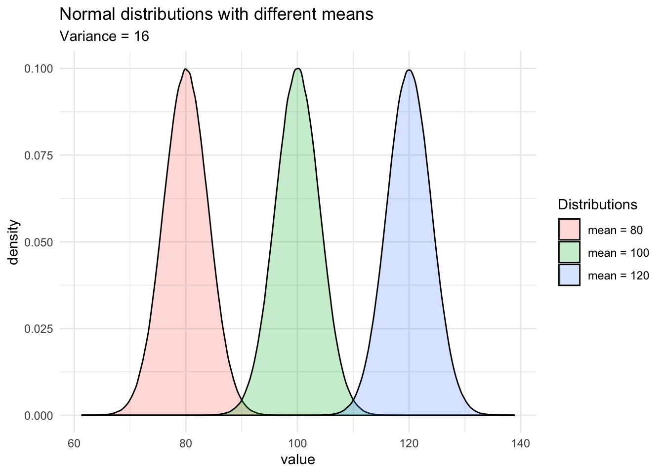
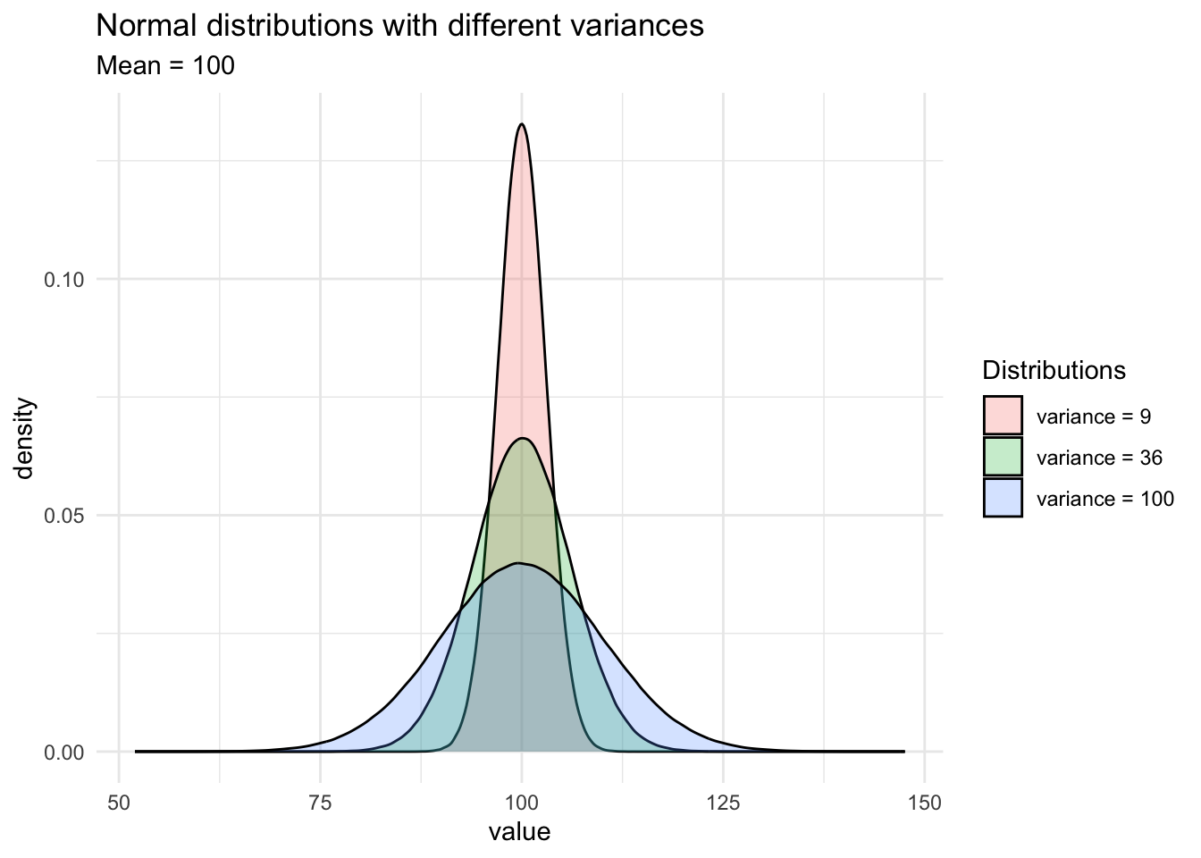
As yous can encounter on the second graph, when the variance (or the standard departure) decreases, the observations are closer to the mean. On the contrary, when the variance (or standard divergence) increases, it is more likely that observations volition be further abroad from the hateful.

A random variable \(Ten\) which follows a normal distribution with a hateful of 430 and a variance of 17 is denoted \(X ~ \sim \mathcal{N}(\mu = 430, \sigma^2 = 17)\).

Nosotros have seen that, although different normal distributions have dissimilar shapes, all normal distributions accept common characteristics:

• They are symmetric, fifty% of the population is above the hateful and l% of the population is beneath the hateful
• The mean, median and mode are equal
• The empirical rule detailed before is applicable to all normal distributions

Probabilities and standard normal distribution

Probabilities and quantiles for random variables with normal distributions are hands found using R via the functions pnorm() and qnorm(). Probabilities associated with a normal distribution can likewise be plant using this Shiny app. However, earlier computing probabilities, we need to learn more than about the standard normal distribution and the \(Z\) score.

Although at that place are infinitely many normal distributions (since there is a normal distribution for every combination of mean and variance), nosotros need only one table to find the probabilities under the normal curve: the standard normal distribution. The normal standard distribution is a special case of the normal distribution where the mean is equal to 0 and the variance is equal to one. A normal random variable \(X\) tin can ever exist transformed to a standard normal random variable \(Z\), a procedure known as "scaling" or "standardization," past subtracting the mean from the observation, and dividing the consequence by the standard deviation. Formally:

\[Z = \frac{X - \mu}{\sigma}\]

where \(Ten\) is the observation, \(\mu\) and \(\sigma\) the mean and standard deviation of the population from which the observation was drawn. So the mean of the standard normal distribution is 0, and its variance is 1, denoted \(Z ~ \sim \mathcal{N}(\mu = 0, \sigma^2 = ane)\).

From this formula, nosotros come across that \(Z\), referred as standard score or \(Z\) score, allows to run into how far away ane specific observation is from the mean of all observations, with the distance expressed in standard deviations. In other words, the \(Z\) score corresponds to the number of standard deviations one observation is away from the hateful. A positive \(Z\) score ways that the specific observation is to a higher place the mean, whereas a negative \(Z\) score ways that the specific observation is below the mean. \(Z\) scores are often used to compare an private to her peers, or more than generally, a measurement compared to its distribution.

For instance, suppose a student scoring 60 at a statistics exam with the hateful score of the course being 40, and scoring 65 at an economics exam with the hateful score of the class being 80. Given the "raw" scores, ane would say that the student performed better in economic science than in statistics. Notwithstanding, taking into consideration her peers, it is clear that the pupil performed relatively meliorate in statistics than in economics. Computing \(Z\) scores allows to take into consideration all other students (i.east., the entire distribution) and gives a ameliorate mensurate of comparison. Let'south compute the \(Z\) scores for the two exams, assuming that the score for both exams follow a normal distribution with the following parameters:

		Statistics	Economics
Mean		twoscore	lxxx
Standard deviation		8	12.5
Pupil's score		60	65

\(Z\) scores for:

• Statistics: \(Z_{stat} = \frac{60 - 40}{8} = two.5\)
• Economic science: \(Z_{econ} = \frac{65 - 80}{12.5} = -one.ii\)

On the one mitt, the \(Z\) score for the examination in statistics is positive (\(Z_{stat} = ii.5\)) which means that she performed better than average. On the other paw, her score for the test in economic science is negative (\(Z_{econ} = -ane.ii\)) which ways that she performed worse than average. Below an analogy of her grades in a standard normal distribution for better comparing:

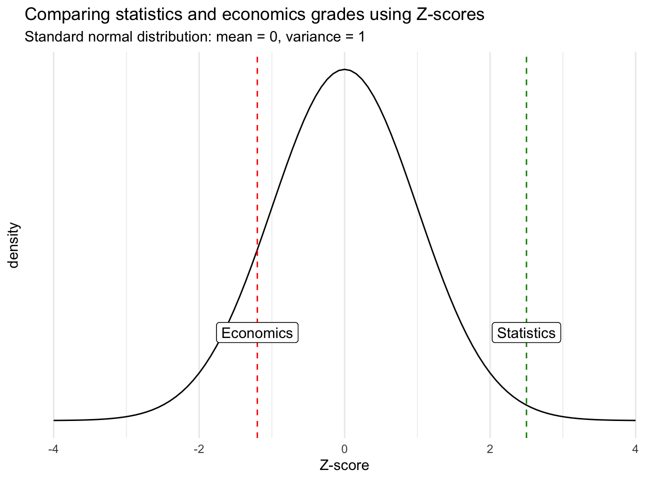
Although the score in economics is better in absolute terms, the score in statistics is actually relatively better when comparing each score inside its own distribution.

Furthermore, \(Z\) score also enables to compare observations that would otherwise be impossible because they take different units for example. Suppose you desire to compare a salary in € with a weight in kg. Without standardization, there is no mode to conclude whether someone is more extreme in terms of her wage or in terms of her weight. Thanks to \(Z\) scores, nosotros can compare two values that were in the starting time place not comparable to each other.

Terminal remark regarding the interpretation of a \(Z\) score: a dominion of thumb is that an observation with a \(Z\) score between -3 and -2 or between ii and iii is considered as a rare value. An observation with a \(Z\) score smaller than -3 or larger than iii is considered as an extremely rare value. A value with any other \(Z\) score is considered equally not rare nor extremely rare.

Areas under the normal distribution in R and by hand

Now that nosotros accept covered the \(Z\) score, nosotros are going to employ information technology to determine the area under the curve of a normal distribution.

Annotation that in that location are several ways to go far at the solution in the following exercises. You may therefore use other steps than the ones presented to obtain the same outcome.

Ex. 1

Permit \(Z\) announce a normal random variable with hateful 0 and standard divergence i, find \(P(Z > 1)\).

We actually wait for the shaded area in the following figure:

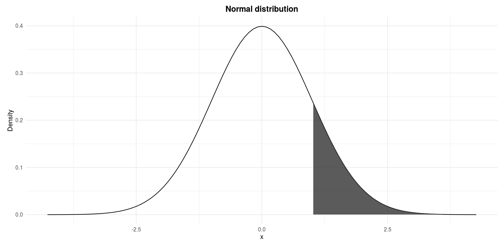
Standard normal distribution: \(P(Z > i)\)

In R

                    pnorm(1,   mean = 0,   sd = 1, # sd stands for standard divergence   lower.tail = Simulated )                  

                    ## [one] 0.1586553                  

Nosotros look for the probability of \(Z\) beingness larger than 1 then we gear up the argument lower.tail = Fake. The default lower.tail = TRUE would give the result for \(P(Z < 1)\). Notation that \(P(Z = 1) = 0\) and so writing \(P(Z > 1)\) or \(P(Z \ge i)\) is equivalent.

By manus

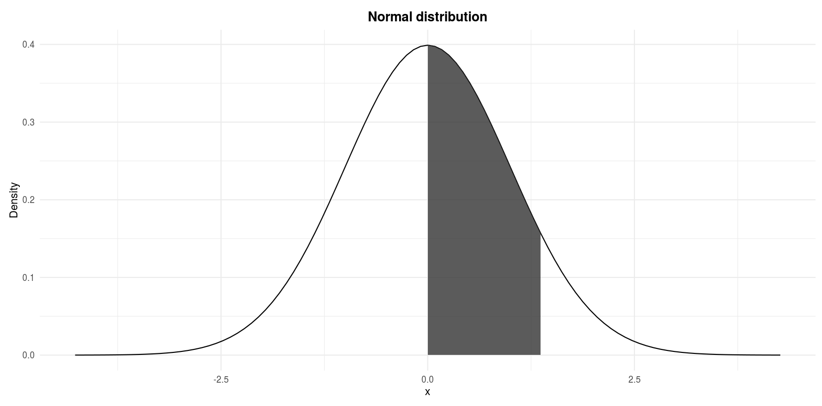
See that the random variable \(Z\) has already a mean of 0 and a standard departure of ane, so no transformation is required. To observe the probabilities past hand, we need to refer to the standard normal distribution table shown below:

Standard normal distribution table (Wackerly, Mendenhall, and Scheaffer 2014).

From the illustration at the top of the table, we see that the values inside the table represent to the surface area under the normal curve above a certain \(z\). Since we are looking precisely at the probability in a higher place \(z = ane\) (since we look for \(P(Z > one)\)), we can simply go on down the first (\(z\)) cavalcade in the tabular array until \(z = 1.0\). The probability is 0.1587. Thus, \(P(Z > 1) = 0.1587\). This is like to what we found using R, except that values in the table are rounded to 4 digits.

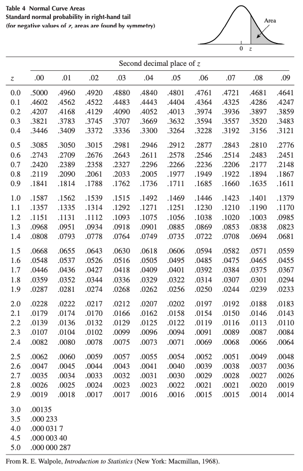
Ex. two

Permit \(Z\) announce a normal random variable with mean 0 and standard departure i, find \(P(−ane \le Z \le ane)\).

We are looking for the shaded area in the following figure:

Standard normal distribution: \(P(−1 \le Z \le 1)\)

In R

                    pnorm(1, lower.tail = Truthful) - pnorm(-ane, lower.tail = TRUE)                  

                    ## [one] 0.6826895                  

Note that the arguments by default for the mean and the standard deviation are hateful = 0 and sd = 1. Since this is what we need, we tin omit them.^ane

By hand

For this practise we continue by steps:

1. The shaded area corresponds to the unabridged surface area under the normal curve minus the two white areas in both tails of the curve.
2. Nosotros know that the normal distribution is symmetric.
3. Therefore, the shaded expanse is the entire area under the bend minus two times the white area in the correct tail of the curve, the white surface area in the right tail of the curve beingness \(P(Z > ane)\).
4. Nosotros also know that the unabridged surface area under the normal curve is 1.
5. Thus, the shaded area is 1 minus ii times \(P(Z > 1)\):

\[P(−1 \le Z \le 1) = one - 2 \cdot P(Z > 1)\] \[= ane - two \cdot 0.1587 = 0.6826\]

where \(P(Z > 1) = 0.1587\) has been found in the previous exercise.

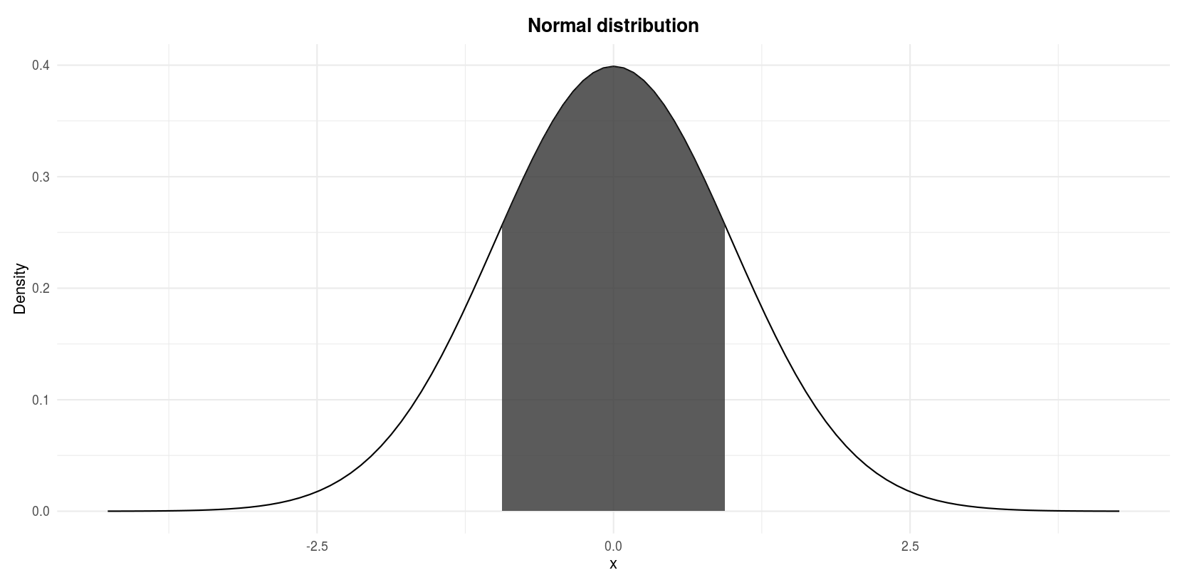
Ex. iii

Let \(Z\) announce a normal random variable with mean 0 and standard departure 1, observe \(P(0 \le Z \le 1.37)\).

We are looking for the shaded area in the post-obit figure:

Standard normal distribution: \(P(0 \le Z \le 1.37)\)

In R

                    pnorm(0, lower.tail = Simulated) - pnorm(1.37, lower.tail = FALSE)                  

                    ## [1] 0.4146565                  

By hand

Over again we keep past steps for this exercise:

1. We know that \(P(Z > 0) = 0.five\) since the entire expanse nether the bend is one, half of it is 0.5.
2. The shaded area is one-half of the unabridged area under the curve minus the expanse from i.37 to infinity.
3. The expanse under the curve from 1.37 to infinity corresponds to \(P(Z > one.37)\).
4. Therefore, the shaded expanse is \(0.5 - P(Z > 1.37)\).
5. To find \(P(Z > ane.37)\), proceed down the \(z\) column in the table to the entry ane.3 and then across the top of the table to the column labeled .07 to read \(P(Z > one.37) = .0853\)
6. Thus,

\[P(0 \le Z \le 1.37) = P(Z > 0) - P(Z > ane.37)\] \[ = 0.v - 0.0853 = 0.4147\]

Ex. iv

Recap the example presented in the empirical dominion: Suppose that the scores of an examination in statistics given to all students in a Belgian university are known to accept a normal distribution with hateful \(\mu = 67\) and standard deviation \(\sigma = 9\). What fraction of the scores lies betwixt lxx and lxxx?

Nosotros are looking for the shaded area in the following figure:

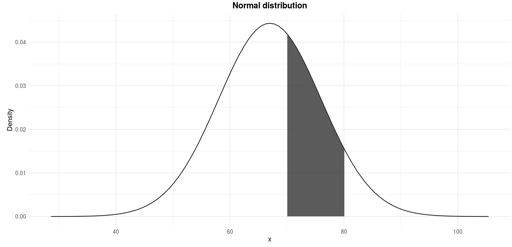
\(P(70 \le X \le lxxx)\) where \(X \sim \mathcal{N}(\mu = 67, \sigma^two = ix^2)\)

In R

                    pnorm(70, mean = 67, sd = 9, lower.tail = Simulated) - pnorm(eighty, hateful = 67, sd = nine, lower.tail = Imitation)                  

                    ## [1] 0.2951343                  

Past mitt

Remind that we are looking for \(P(70 \le Ten \le 80)\) where \(X \sim \mathcal{Due north}(\mu = 67, \sigma^2 = nine^2)\). The random variable \(10\) is in its "raw" format, pregnant that it has not been standardized yet since the hateful is 67 and the variance is \(9^2\). We thus demand to first use the transformation to standardize the endpoints 70 and fourscore with the following formula:

\[Z = \frac{X - \mu}{\sigma}\]

After the standardization, \(x = lxx\) becomes (in terms of \(z\), so in terms of deviation from the hateful expressed in standard deviation):

\[z = \frac{lxx - 67}{ix} = 0.3333\]

and \(10 = 80\) becomes:

\[z = \frac{80 - 67}{nine} = one.4444\]

The figure above in terms of \(X\) is now in terms of \(Z\):

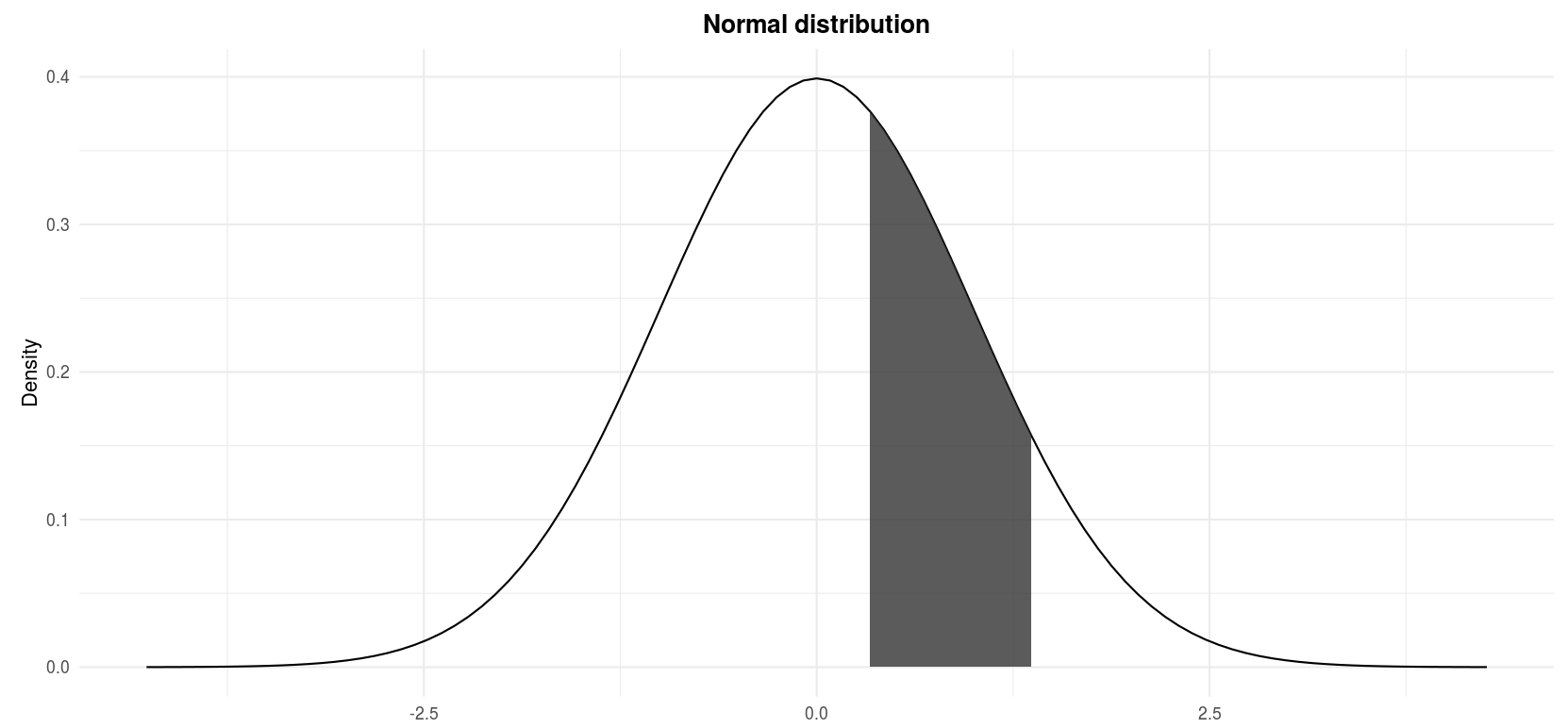
\(P(0.3333 \le Z \le 1.4444)\) where \(Z \sim \mathcal{N}(\mu = 0, \sigma^2 = ane)\)

Finding the probability \(P(0.3333 \le Z \le 1.4444)\) is similar to exercises 1 to 3:

1. The shaded area corresponds to the area under the curve from \(z = 0.3333\) to \(z = 1.4444\).
2. In other words, the shaded area is the area under the bend from \(z = 0.3333\) to infinity minus the expanse nether the bend from \(z = 1.4444\) to infinity.
3. From the tabular array, \(P(Z > 0.3333) = 0.3707\) and \(P(Z > 1.4444) = 0.0749\)
4. Thus:

\[P(0.3333 \le Z \le 1.4444)\] \[= P(Z > 0.3333) - P(Z > 1.4444)\] \[= 0.3707 - 0.0749 = 0.2958\]

The difference with the probability found using in R comes from the rounding.

To conclude this do, we can say that, given that the hateful scores is 67 and the standard deviation is 9, 29.58% of the students scored between 70 and 80.

Ex. 5

See another instance in a context hither.

Why is the normal distribution so crucial in statistics?

The normal distribution is important for 3 primary reasons:

• Some statistical hypothesis tests assume that the data follow a normal distribution
• The central limit theorem states that, for a large number of observations (usually \(n > 30\)), no matter what is the underlying distribution of the original variable, the distribution of the sample ways (\(\overline{10}_n\)) and of the sum (\(S_n = \sum_{i = 1}^n X_i\)) may exist approached by a normal distribution (Stevens 2013)
• Linear and nonlinear regression assume that the residuals are usually-distributed (for modest sample sizes)

Information technology is therefore useful to know how to test for normality in R, which is the topic of side by side sections.

How to test the normality assumption

Every bit mentioned above, some statistical tests crave that the information follow a normal distribution, or the event of the exam may be flawed.

In this section, we show 4 complementary methods to determine whether your data follow a normal distribution in R.

Histogram

A histogram displays the spread and shape of a distribution, so it is a good starting point to evaluate normality. Let's take a wait at the histogram of a distribution that nosotros would await to follow a normal distribution, the height of 1,000 adults in cm:

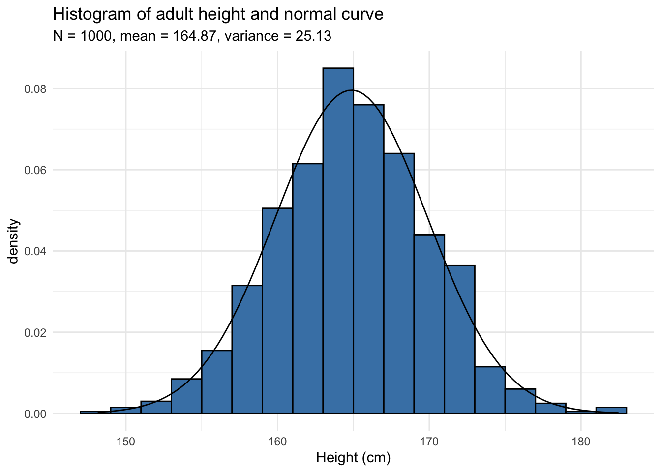
The normal curve with the corresponding mean and variance has been added to the histogram. The histogram follows the normal bend so the data seems to follow a normal distribution.

Beneath the minimal code for a histogram in R with the dataset iris:

                data(iris) hist(iris$Sepal.Length)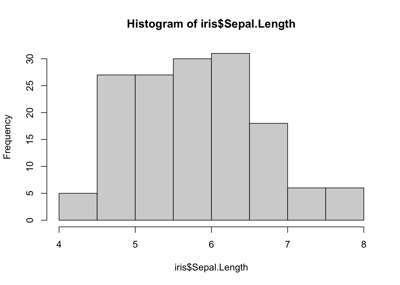              

In {ggplot2}:

                ggplot(iris) +   aes(10 = Sepal.Length) +   geom_histogram()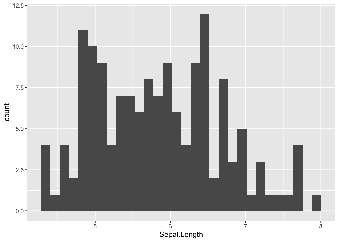              

Histograms are however not sufficient, peculiarly in the example of modest samples considering the number of bins profoundly change its appearance. Histograms are not recommended when the number of observations is less than 20 because it does not e'er correctly illustrate the distribution. Run into 2 examples below with dataset of 10 and 12 observations:

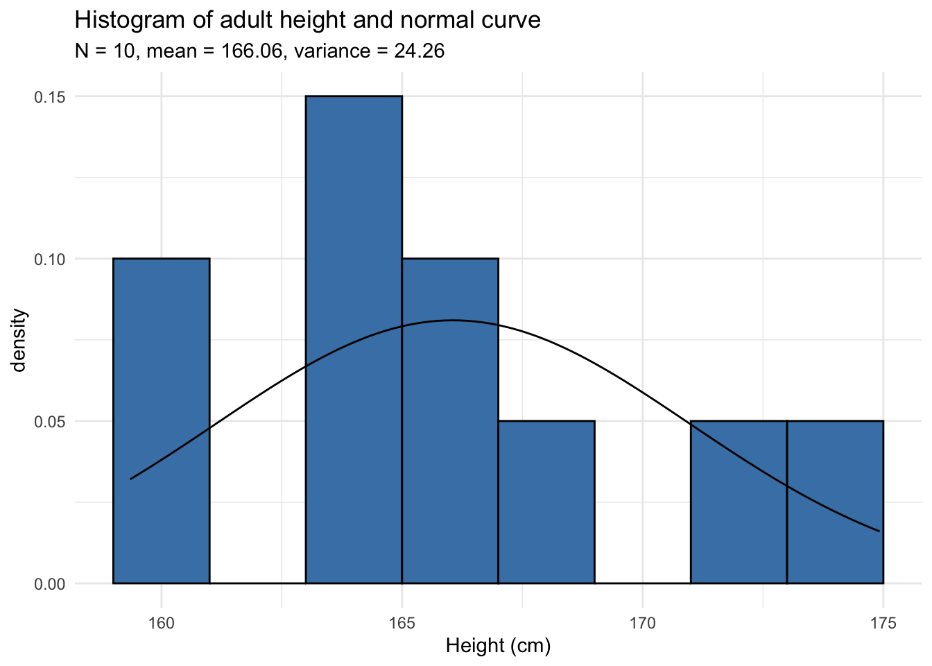
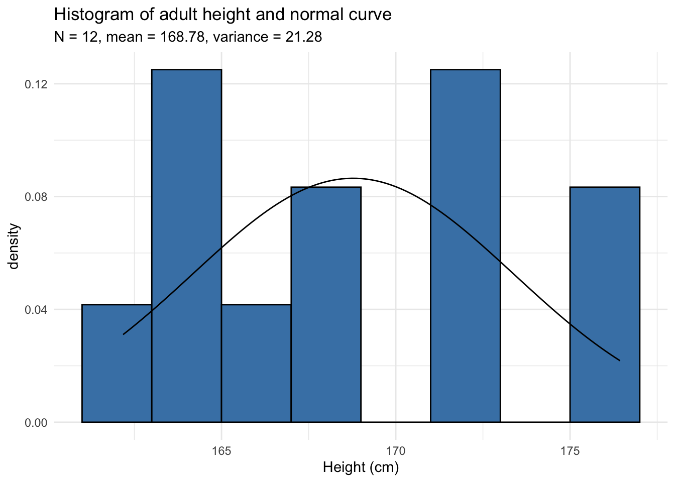
Can you tell whether these datasets follow a normal distribution? Surprisingly, both follow a normal distribution!

In the remaining of the article, nosotros will utilise the dataset of the 12 adults. If you lot would like to follow my lawmaking in your own script, here is how I generated the data:

                set up.seed(42) dat_hist <- data.frame(   value = rnorm(12, mean = 165, sd = 5) )              

The rnorm() role generates random numbers from a normal distribution (12 random numbers with a hateful of 165 and standard deviation of v in this case). These 12 observations are so saved in the dataset called dat_hist under the variable value. Notation that set.seed(42) is important to obtain the exact same data every bit me.²

Density plot

Density plots also provide a visual judgment near whether the information follow a normal distribution. They are similar to histograms as they also allow to analyze the spread and the shape of the distribution. However, they are a smoothed version of the histogram. Hither is the density plot fatigued from the dataset on the height of the 12 adults discussed higher up:

                plot(density(dat_hist$value))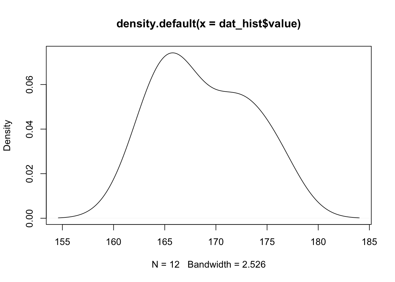              

In {ggpubr}:

                library("ggpubr") # bundle must be installed start ggdensity(dat_hist$value,   master = "Density plot of adult height",   xlab = "Height (cm)" )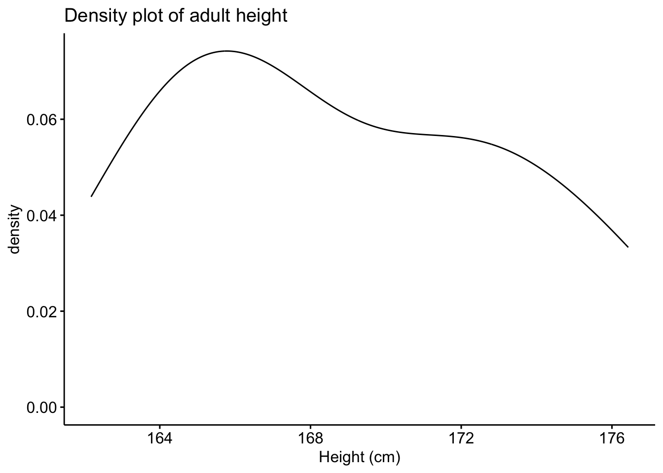              

Since it is difficult to test for normality from histograms and density plots just, it is recommended to corroborate these graphs with a QQ-plot. QQ-plot, also known as normality plot, is the third method presented to evaluate normality.

QQ-plot

Like histograms and density plots, QQ-plots allow to visually evaluate the normality assumption. Here is the QQ-plot drawn from the dataset on the height of the 12 adults discussed to a higher place:

                library(motorcar) qqPlot(dat_hist$value)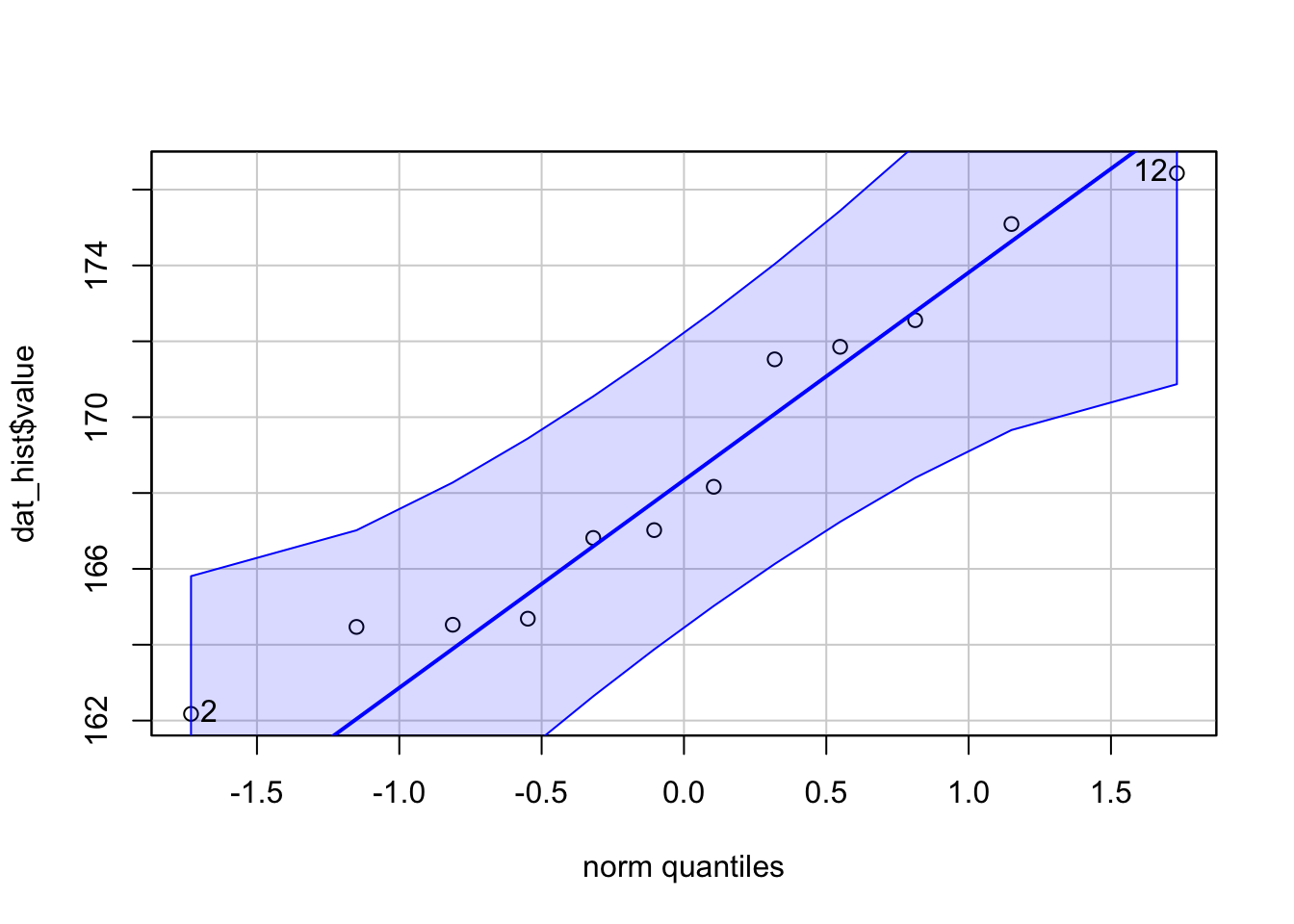              

                ## [1] 12  2              

In {ggpubr}:

                library(ggpubr) ggqqplot(dat_hist$value)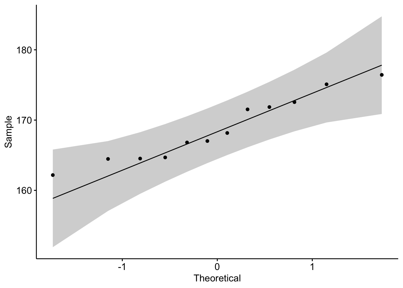              

Instead of looking at the spread of the data (every bit it is the example with histograms and density plots), with QQ-plots we just need to ascertain whether the information points follow the line (sometimes referred as Henry'southward line).

If points are shut to the reference line and inside the conviction bands, the normality assumption can be considered equally met. The bigger the deviation between the points and the reference line and the more they lie exterior the conviction bands, the less likely that the normality status is met. The height of these 12 adults seem to follow a normal distribution because all points lie within the confidence bands.

When facing a non-normal distribution every bit shown by the QQ-plot beneath (systematic departure from the reference line), the first step is usually to apply the logarithm transformation on the data and recheck to meet whether the log-transformed data are normally distributed. Applying the logarithm transformation can be done with the log() role.

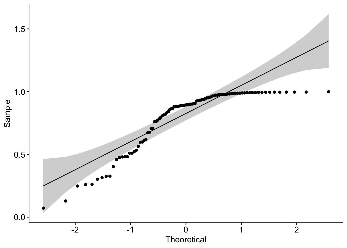
Note that QQ-plots are as well a convenient way to assess whether residuals from linear regression follow a normal distribution.

Normality test

The iii tools presented above were a visual inspection of the normality. Nevertheless, visual inspection may sometimes be unreliable so information technology is besides possible to formally test whether the information follow a normal distribution with statistical tests. These normality tests compare the distribution of the data to a normal distribution in order to assess whether observations show an important deviation from normality.

The ii most common normality tests are Shapiro-Wilk's test and Kolmogorov-Smirnov examination. Both tests accept the same hypotheses, that is:

• \(H_0\): the data follow a normal distribution
• \(H_1\): the information do not follow a normal distribution

Shapiro-Wilk test is recommended for normality test as it provides amend power than Kolmogorov-Smirnov exam.³ In R, the Shapiro-Wilk test of normality can exist done with the function shapiro.test():^iv

                shapiro.test(dat_hist$value)              

                ##  ##  Shapiro-Wilk normality test ##  ## information:  dat_hist$value ## West = 0.93968, p-value = 0.4939              

From the output, nosotros see that the \(p\)-value \(> 0.05\) implying that we do not reject the zip hypothesis that the information follow a normal distribution. This test goes in the same direction than the QQ-plot, which showed no significant divergence from the normality (as all points lied within the confidence bands).

It is of import to notation that, in practise, normality tests are oft considered every bit too conservative in the sense that for large sample size (\(n > 50\)), a minor deviation from the normality may cause the normality condition to be violated. A normality test is a hypothesis exam, and so as the sample size increases, their chapters of detecting smaller differences increases. So as the number of observations increases, the Shapiro-Wilk test becomes very sensitive even to a minor departure from normality. As a consequence, it happens that according to the normality examination the data do not follow a normal distribution although the departures from the normal distribution is negligible then the data could in fact be considered to follow approximately a normal distribution. For this reason, information technology is oft the case that the normality condition is verified based on a combination of all methods presented in this article, that is, visual inspections (with histograms and QQ-plots) and a formal inspection (with the Shapiro-Wilk test for instance).

I personally tend to prefer QQ-plots over histograms and normality tests so I do non have to bother nearly the sample size. This commodity showed the different methods that are available, your choice volition of grade depends on the type of your data and the context of your analyses.

Thanks for reading. I promise the article helped you to acquire more nigh the normal distribution and how to test for normality in R.

Every bit always, if you lot take a question or a suggestion related to the topic covered in this article, please add together it every bit a comment so other readers can benefit from the give-and-take.

References

Stevens, James P. 2013. Intermediate Statistics: A Modern Approach. Routledge.

Wackerly, Dennis, William Mendenhall, and Richard L Scheaffer. 2014. Mathematical Statistics with Applications. Cengage Learning.

Liked this post?

Become updates every fourth dimension a new commodity is published.
No spam and unsubscribe anytime.

Share on:

How To See If Data Is Normally Distributed,

Source: https://statsandr.com/blog/do-my-data-follow-a-normal-distribution-a-note-on-the-most-widely-used-distribution-and-how-to-test-for-normality-in-r/

Posted by: shiresplesn1976.blogspot.com

Share this post